How much money does the economy need?
Prof. Dr. Urs Birchler explains the important quantitative theory of monetary policy with examples and graphs. It is one of the most important formula to explain money policy since the Middle Ages.

How much money does the economy need?
First, a story:
Anna and her mother sell apples at the market. In the evening she reviewed her day’s business: She sold fifty kilos of apples for 6 francs per kilo. That yielded 300 francs, the amount she had in her cashbox. For Anna, turnover equals the quantity sold, Q, times the price, P.
Bored during quiet spells at the market, Anna had idly written her name on the banknotes she’d taken in that day. A week later, again at her stand, she was amazed when a customer paid with a bill that bore her signature! She had spent that money and it had circulated through the economy and returned to her.
This led Anna to think that while an apple can only be eaten once, a banknote obviously can be used a multitude of times. And the more a bank note changes hands, she thought, the fewer total bills are needed.
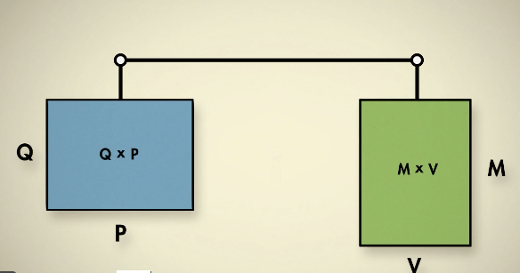
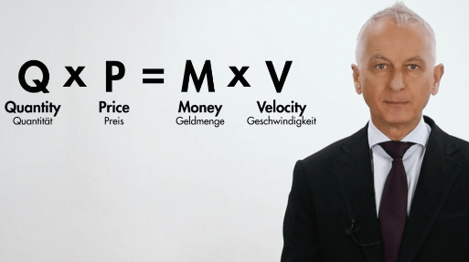
She took out her pen and made a note of this relationship: Quantity (Q) times price (P) equals the supply of money (M) times the frequency with which that money is spent (V, for velocity). Both sides of the equation measure turnover—the first from the goods side, and then from the monetary or money side.
This formula is known as the quantity equation. Ancient Chinese scholars already formulated it twenty-five hundred years ago. Indeed, the effects of too little or too much money in the economy has been an issue throughout history. The quantity equation is easy to grasp. It functions like a scale: too much weight on one side or the other swings the balance to surplus or shortage.
Quantitiy times Price equals Money Supply times Velocity
During the Middle Ages in Europe, the mines were exhausted, leading to a scarcity of metals suitable for minting. Added to that, Europe’s money was flowing to the Orient to buy spices and silks, making it necessary to mint coins from ever lower quality metals, thin, and often marked only on one side. But this didn’t solve the money shortage (-M) in Europe. Traders had to lower their prices (-P) or sell less (-Q). Some historians argue that the scarcity of money actually led to the Dark Ages.
But an antidote for money scarcity soon appeared: creative bankers like the Medici in Florence invented cashless payments, for example, by means of commercial bills of trade. These promises of payment allowed money to circulate virtually, to go wherever it was needed, which increased the velocity of circulation (+V). This enabled traders to sell more goods or ask higher prices and Europe’s economy flourished (+Q).
The scarcity of money was quickly forgotten. Christopher Columbus landed in the Americas in 1492 and boatloads of gold and silver soon began arriving in Spain and circulating throughout Europe. This windfall (++M) increased Europe’s money supply by at least a factor of 10, as the total economy grew (+Q, by about 1.66). The Renaissance was fed by these riches.
But prices also rose sharply in Europe (++P) over the next hundred and fifty years. This led the Spanish monk Martin de Azpilcueta to formulate the relationship between a rising money supply and rising prices. Two thousand years after the Chinese, he formalized the quantity equation for Europe.
Inflation and Deflation
The end of First World War, a hundred years ago, produced an extreme illustration of the quantity equation at work. A defeated Germany urgently needed money to rebuild. The country’s central bank, the Reichsbank, fired up the printing presses, increasing the money supply dramatically (++M, arrow 1 on the right).
The economy surged but very quickly everything was a lot more expensive. Hyperinflation soon took hold and the value of money spiraled out of control (+M, +P, +M, +P, +M). Suddenly a loaf of bread cost twice as much in the evening as it had in the morning. Spending went on a furious pace and money changed hands like a hot potato.
The velocity of circulation soared but so did prices. The economy collapsed and bank notes became worthless. A bread cost a billion marks but bakers would sell. All over Germany, printing press struggled to keep pace with demand for bank notes. But the couldn’t keep pace with money’s plummeting loss of value. The economy collapsed and money became a worthless toy.
In time, the pendulum swung the other way: deflation followed inflation. After the stock market crash of 1929, banks collapsed and the world’s central banks decided to severely choke off the money supply (--M). Prices and wages fell sharply (-P) and the economy shriveled (-Q). The Great Depression hit its low point in 1933. Only the depreciation of the major currencies against gold enabled the central banks to remedy the lack of money (+M). The global economy began to recover.
The quantity equation is always valid
More recently, in 2007 the world’s big banks held mountains of worthless real estate credits. Banks no longer trusted one another and they stopped lending to each other, bringing the velocity of circulation to a stop (-V). Central banks, fearing an imminent economic collapse, began to pump massive amounts of money into the banking system (+++M). They managed to avoid the worst but money is still moving only sluggishly through the economy (---V). The vast money supply is a sleeping giant and when money starts flowing again, inflation awaits.
The quantity equation helps to describe the economic and monetary dynamics of inflation and deflation. But it can’t tell us why; it doesn’t explain the causes and effects of these developments.
The central banks try to help the economy by adjusting the money supply (the bright M), but they don’t know exactly what effects their efforts will have on the other three big economic factors — the real economy (which refers to the nonfinancial parts of the economy), price levels and the velocity of circulation. Often, short-term effects differ from long-term developments.
The relationships between these four decisive factors don’t follow any natural laws. They are driven by policy decisions made by people. And they don’t always interact the same way in different circumstances. Only the equation remains constant.